Study Participants
Ethical approval was obtained through the Children’s Health Ireland Research Ethics Committee (REF: rec-398-24). MRI datasets from GE Signa Architect 3T MRI scanner were divided into 3 groups: (1) no evident pathology, (2) subtle pathology and (3) major pathology. T2 fast spin echo (FSE) brain scans, both ARDL reconstructed and the corresponding conventionally reconstructed version (ORIG), were anonymised and exported. ARDL images acquired were set to ‘High’ noise removal. DICOM headers were edited to allow blinding of the image type for the subsequent qualitative analysis. Unique accession numbers were created for each patient, with each ARDL and conventional sequence labelled A or B.
Quantitative Analysis
Post-Processing
The FMRIB Software Library (FSL) was used for post-processing the images [10]. Automated programs run on FSL through Python included a brain extraction tool (BET) and an automated segmentation tool (FAST) to segement the images into grey matter (GM), white matter (WM) and cerebrospinal fluid (CSF), while correcting bias field inhomogeneities.
SNR & CNR Quantification
A Python function calculated SNR for both ARDL and ORIG subsets in groups 1,2 and 3. The final images used for mean signal extraction were acquired by multiplying the brain extracted data, inverse bias field data and binary tissue segmented maps. Pixel data from the processed scans were extracted from each binary segmented tissue mask (GM, WM, CSF). Noise was calculated from the pre-processed sequences. SNR was calculated for each tissue type as the ratio of mean signal to image noise. Using the same values, CNR between tissue types was also analysed for both image reconstruction types.
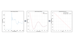
Gibbs Ringing Quantification
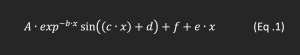
An interactive Python function was used for manual identification of the ringing pattern (Fig .1). Three metrics were obtained from the analysis of the oscillating wave: maximum oscillation amplitude (the first occurrence of artificially high signal in the ringing pattern), damping factor, (b constant seen in Eq. 1) and decay rate, calculated by performing a logarithmic transformation of the extracted amplitudes, and determining the rate of decay of the amplitudes (Fig .3).
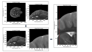
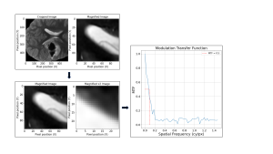
Spatial Resolution
To analyse the spatial resolution in both ARDL and ORIG sequences, a method similar to Gibbs Ringing identification was employed (Fig. 4). Manual localisation of a ventricle horn facilitated the isolation of a suitable slanted edge. An SFR repository from GitHub was employed [11], providing a comprehensive set of Python scripts designed for SFR determination of a slanted edge.
Qualitative Analysis
Questionnaires were created for groups 1,2 and 3. Radiologists compared images A to B, scoring the images according to the Likert scale on the images noise level, spatial resolution, anatomy/lesion conspicuity and artefact presence. The comparison of A to B used scores 4-5 for A better than B, 1-2 for A worse than B, and 3 for equivalence.
A binary logistic regression classifier was used to predict the likelihood of sequence A being ARDL reconstructed, based on the radiologists’ scores [12,13]. The dependent variable is whether sequence A was ARDL reconstructed, and the independent variables consist of the radiologist scores for each image quality metric (noise level, spatial resolution, anatomy/lesion conspicuity and artefact presence). The independent variables were used to estimate the likelihood that sequence A was generated through ARDL reconstruction.
To evaluate the classifiers performance, accuracy, F1 score and independent variable coefficients were the metrics employed. High accuracy and F1 scores indicate the radiologist’s scoring follow the expected values of 4 or higher for ARDL reconstructed images. Independent variable coefficients represent the impact of each image quality metric (noise, spatial resolution, artefact and detectability) on the classifiers predicted reconstruction method.