For this study, a CCR (Credence Cartridge Radiomics) phantom, analogous to the one used by Mackin et al. [8], was used, as shown in Figure 1.  The phantom consists of ten materials enclosed in an acrylic casing, specifically: plaster, wood, cork, rubber, polyurethane, PMMA (a highly transparent thermoplastic polymer), and ABS (Acrylonitrile Butadiene Styrene) at 20%, 30%, 40%, and 50%.

Fig 1: CCR phantom.

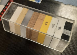
Image acquisition was performed using the Gemstone Spectral Imaging (GSI) computed tomography scanner from General Electric. A total of seven series were acquired in fast kV-switching CT (fsCT) mode and three in polychromatic tube CT (pCT) mode. For repeatability assessment, identical series were acquired. Monoenergetic and virtual unenhanced reconstructions were compared. For reproducibility analysis, monoenergetic (ME) and kV-Like reconstructions from fsCT were compared with their corresponding kV acquisitions in pCT. Figure 2 presents a schematic representation of the methodology employed in this study.  

Fig 2: Methodology for the robustness assessment.

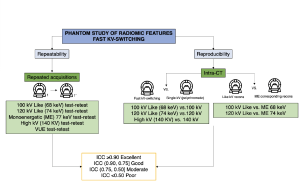
All acquisitions were performed at 250 mA, with a pitch value of 1 and a slice thickness of 1.25 mm. When operating at a fixed tube voltage, acquisitions were performed at 100 kV, 120 kV, and 140 kV. In the case of dual-energy imaging, the tube operated in rapid switching mode between two voltages: 80/140 kV.

Comparisons were made between kV-Like and monoenergetic (ME) reconstructions. The ME reconstruction generates an image simulating X-ray acquisition at a single energy level rather than a polychromatic beam. ME images were analyzed at 68 keV and 74 keV. The kV-Like reconstruction simulates the tube operating at a single voltage while using fsCT. Additionally, a virtual unenhanced image (VUE) was reconstructed. Comparisons between kV-Like and ME reconstructions were performed following the manufacturer’s guidelines.

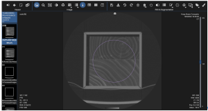
For image management and radiomic feature extraction, the Quibim Precision platform was used. Segmentation for feature extraction and calculations were processed with the same software. Specifically, ten volumes of interest (VOIs) were defined in each series, one for each material in the phantom. The VOIs had a cylindrical geometry with a radius of 43 mm and a length of 20 mm. Figure 3 presents a screenshot from the image viewer, showing an axial slice of the wood sample with the region of interest delineated in violet.  

Fig 3: Screenshot of the Quibim Precision viewer of an axial section of the wood with the ROI highlighted in purple.

Subsequently, radiomic feature extraction was performed. The platform utilizes proprietary extraction software based on the Pyradiomics library in Python. Prior to feature calculation, image grayscale normalization was applied, outlier values were removed, voxel dimensions were resampled to isotropic (1×1×1 mm³), and the unit distance to the nearest neighbor was set. A total of 110 radiomic features were extracted, categorized into different families: shape, first-order, and second-order (Gray Level Co-occurrence Matrix, Gray Level Run Length Matrix, Gray Level Size Zone Matrix, Gray Level Dependence Matrix, and Neighboring Gray Tone Difference Matrix). Notably, the 19 shape-related features were excluded from this study, as the phantom geometry was predefined and identical across all acquisitions, thus providing no relevant information regarding feature robustness.

To assess feature robustness, the intraclass correlation coefficient (ICC) was used. This metric evaluates the consistency of repeated measurements concerning total variability [9] and is classified as excellent for values above 0.9, good between 0.75 and 0.9, moderate between 0.5 and 0.75, and poor when below 0.5. These calculations were performed using R software.